Why Use Adaptive Generalized Elliptical Slice Sampling?

Given the vast amount of MCMC methods available, one has to wonder what makes adaptive generalized elliptical slice sampling^[1] (AGESS) even worth considering. Concisely, what makes this method desirable is that (1) you can achieve nearly dimension-free mixing times in optimal scenarios, (2) it does not require the target distribution to be differentiable, and (3) it is able to traverse complex target distributions that are multimodal or have highly localized features. We will start by first exploring the efficiency claims, and then will illustrate the performance of AGESS on a multimodal distribution.

Download this page as a Jupyter notebook

(Almost) Dimension-Free Mixing Times

In the manuscript^[1], we prove that an optimally specified elliptical slice sampler can achieve mixing times that scale logarithmically ($\mathcal{O}(\log(P))$) with the dimension of the target distribution (when we have a Gaussian target distribution). Moreover, we prove that measures of the multivariate effective sample size (empirical measures for assessing the mixing time) are dimension independent when the target distribution is a Gaussian distribution. In comparison, an optimally tuned adaptive random walk is only able to achieve mixing times that are $\mathcal{O}(P)$^[3], while Hamiltonian Monte Carlo (under optimal conditions and a warm start) has a gradient complexity (defined as the mixing time multiplied by the number of gradient evaluations per iteration) of $\mathcal{O}(P^{1/4})$^[2]–-that is, both sampling schemes scale polynomially with dimension. AGESS is a promising sampler that scales extremely well with the dimension of the target distribution.

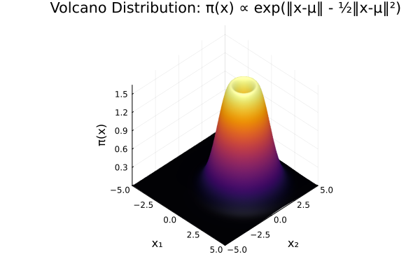
The fundamental question becomes: does this scaling property only hold with Gaussian target distributions? Empirical evidence suggests that this is not the case, and that similar mixing times can be obtained under a broader class of target distributions. Here we will illustrate that we can obtain seemingly dimension-free effective sample size estimates on the Volcano distribution–-an elliptical, but not monotonically decreasing, contoured distribution. We will define a non-central Volcano distribution as follows:

\[\pi(\mathbf{x}) \propto \exp\left\{\lVert \mathbf{x} - \boldsymbol{\mu} \rVert - \frac{1}{2}\lVert \mathbf{x}- \boldsymbol{\mu} \rVert^2 \right\}.\]

Let's start by visualizing the Volcano distribution in two dimensions.

using Plots, LinearAlgebra, Turing, Random, MCMCChains
using AdaptEllipticalSliceSampler, EllipticalSliceSampling, AdvancedMH

# Volcano distribution (unnormalized): μ(x) ∝ exp{‖x‖ - ½‖x‖²}
function Volcano_density(x::AbstractVector{<:AbstractFloat}, μ::AbstractVector{<:AbstractFloat},
                         ph::AbstractVector{<:AbstractFloat})
    @. ph = x - μ
    pdf = norm(ph)
    pdf -= 0.5 * norm(ph)^2

    return exp(pdf)
end

# Function for graphing (buffers reused across the 400×400 grid instead of
# allocating three new vectors on every call)
const volcano_x = zeros(2)
const volcano_μ = [1.0, 1.0]
const volcano_ph = zeros(2)
function Volcano(x1, x2)
    volcano_x[1] = x1
    volcano_x[2] = x2
    return Volcano_density(volcano_x, volcano_μ, volcano_ph)
end

grid1 = range(-5, 5; length=400)

surface(
    grid1,
    grid1,
    Volcano;
    camera=(45, 40),
    color=:inferno,
    colorbar=false,
    xlabel="x₁",
    ylabel="x₂",
    zlabel="π(x)",
    title="Volcano Distribution: π(x) ∝ exp(‖x-μ‖ - ½‖x-μ‖²)",
)

To study the sampling efficiency of AGESS, let's compare how the effective sample size changes as we increase the dimension of the Volcano ($P = 2, 10, 50$). Here we will compare the performance of AGESS against alternative samplers such as (1) adaptive random walk, (2) Metropolis Hastings, and (3) elliptical slice sampling^[4] (with a misspecified prior of $\mathcal{N}(\mathbf{0},\mathbf{I})$, but same target distribution). While we would like to compare the sampling performance to gradient-based methods (such as HMC), the target distribution is non-differentiable at $\boldsymbol{\mu}$. Let's start by constructing a Turing model so that we can easily compare the various samplers.

# Volcano distribution as a Turing model: π(x) ∝ exp{‖x-μ‖ - ½‖x-μ‖²}
# Construct it in a way such that the prior is not a good estimate of the posterior
@model function Volcano_turing(μ::AbstractVector{<:AbstractFloat})
    x ~ MvNormal(zeros(length(μ)), I)
    Turing.@addlogprob! norm(x - μ) - 0.5*norm(x - μ)^2 + 0.5*norm(x)^2
end

Volcano_turing (generic function with 2 methods)

Now we can set up a quick simulation to compare the performance. We will run the Metropolis Hastings sampler for $P \times 50000$ iterations, discarding the initial $P \times 25000$ iterations due to burn-in. The rest of the Markov chains will be run for $P \times 10000$ iterations, discarding the initial $P \times 5000$ iterations due to burn-in. We will compare the median one-dimensional ESS (provided as standard output) across the varying dimension of target distributions and various samplers.

function run_comparison(P::Int; seed=123)
    μ = ones(P)
    model = Volcano_turing(μ)

    n_MCMC = P * 10_000
    burn_in = P * 5_000
    post_burn_in = n_MCMC - burn_in

    median_ess(chain) = median(MCMCChains.ess(chain).nt.ess)
    results = Dict{String,Float64}()

    # AGESS
    AGESS_sampler = AGESSSampler(model, n_MCMC)
    chain_AGESS = sample(Xoshiro(seed), model, AGESS_sampler, n_MCMC; progress=false)
    # Divide by the length of chain after burnin
    results["AGESS"] = median_ess(chain_AGESS[(burn_in + 1):end, :, :]) / post_burn_in

    # Elliptical slice sampling
    chain_ESS = sample(Xoshiro(seed), model, Turing.ESS(), n_MCMC; progress=false,
                       chain_type=MCMCChains.Chains)
    # Divide by the length of chain after burnin
    results["ESS"] = median_ess(chain_ESS[(burn_in + 1):end, :, :]) / post_burn_in

    # Metropolis-Hastings
    chain_MH = sample(Xoshiro(seed), model, MH(), 5*n_MCMC; progress=false,
                      chain_type=MCMCChains.Chains)
    # Divide by the length of chain after burnin
    results["MH"] = median_ess(chain_MH[(5*burn_in + 1):end, :, :]) / (5*post_burn_in)

    # Adaptive random walk
    ram = externalsampler(RobustAdaptiveMetropolis(); unconstrained=false)
    chain_ARW = sample(Xoshiro(seed), model, ram, n_MCMC; num_warmup=burn_in,
                       discard_initial=burn_in, progress=false, chain_type=MCMCChains.Chains)
    # Divide by the length of chain after burnin
    results["ARW"] = median_ess(chain_ARW) / post_burn_in

    return results
end

Ps = [2, 10, 50]
samplers = ["AGESS", "ESS", "ARW", "MH"]
all_results = Dict(P => run_comparison(P) for P in Ps)

p = plot(;
    yscale = :log10,
    xlabel="Dimension (P)",
    ylabel="Median ESS per Iteration",
    xscale=:log10,
    xticks=(Ps, string.(Ps)),
    yticks=[1, 0.1, 0.01, 0.001, 0.0001],
    legend=:outertopright,
    title="Sampler Efficiency on the Volcano Distribution",
)
for s in samplers
    plot!(p, Ps, [all_results[P][s] for P in Ps]; label=s, marker=:circle, lw=2)
end
p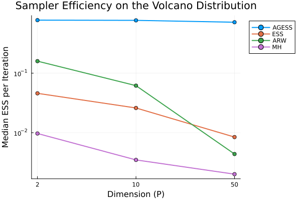

First, note that the y-axis of the plot above is on a logarithmic scale. We can see that as the dimension of the target distribution increases, the effective sample size per iteration significantly decreases for most samplers (adaptive random walk (ARW), Metropolis Hastings (MH), and elliptical slice sampler (ESS)). It is crucial to realize that in this case, even though the elliptical slice sampler has the same target distribution as the other samplers, it is not assuming a Gaussian prior that is centered at $\boldsymbol{\mu}$. Instead, it assumes that the prior is a Gaussian prior that is centered at the origin; that is, a prior that has a significant mismatch with the target distribution. As the dimension of the target distribution grows, this discrepancy leads to larger losses in sampling efficiency. Crucially, AGESS starts with this same (bad) prior; but, through online learning of the target distribution, it is able to learn the geometry of the target distribution, leading to more efficient sampling. This is precisely why elliptical slice samplers tend to perform poorly in high-dimensional settings–-a slight mismatch between the prior and the target will lead to significant losses in sampling efficiency, leading to the need for adaptation.

Key Takeaway: AGESS can offer a significantly faster mixing Markov chain than common alternative samplers, especially when the target distribution is elliptically contoured.

Performance on Complex Target Distributions

Although we have demonstrated that AGESS is extremely efficient when the target distributions that have nice elliptical contours, a perhaps more important question is: what happens when we target more complex target distributions? To answer this question, perhaps it is first beneficial to explicitly define some cases of complex target geometry:

1. Multimodal Distributions (Examples considered: Twin Banana, Deep GP)
2. Distributions with locally-varying curvature (Examples considered: Banana, High-Dimensional Regression with Horseshoe prior, Deep GP, Bayesian Neural Networks).

Most samplers struggle with multimodal distributions; gradient-based samplers are prone to getting stuck in local modes and adaptive random walks are also likely to get stuck if the step size is not sufficiently large. However, elliptical slice samplers are capable of making relatively large global moves, thereby allowing it to traverse multimodal distributions. To ensure that this property holds in AGESS, we randomly mix in non-adaptive kernels, which allow us to traverse these multimodal distributions while still taking advantage of adaptation.

When dealing with distributions that have locally-varying curvature, elliptical slice samplers are optimal candidates as they locally adapt to the geometry by shrinking the proposal region on the ellipse until a suitable next move is found. Similarly, AGESS retains this key property, and has been shown to reliably handle target distributions with localized features. Alternatively, gradient-based methods that only have global tuning parameters can suffer from divergent transitions, causing unreliable posterior inference.

To illustrate the performance of AGESS on complex target distributions, we consider a two-dimensional target distribution with varying geometry, used in the Turing.jl documentation. The target distribution can be specified through the following hierarchical representation:

\[s^2 \sim IG(2,3) \qquad m \sim \mathcal{N}(0, s^2);\]

\[x_i \sim \mathcal{N}(m + 5(\sin(m) + \cos(m)), s^2).\]

Let's start by defining this model using the Turing model.

@model function complex_target(x)
    s² ~ InverseGamma(2, 3)
    m ~ Normal(0, sqrt(s²))
    bumps = sin(m) + cos(m)
    m = m + 5 * bumps
    for i in eachindex(x)
        x[i] ~ Normal(m, sqrt(s²))
    end
    return s², m
end

complex_target (generic function with 2 methods)

Since the target is only two-dimensional, we are able to visualize how a sampler is able to traverse and explore the target distribution. Here, we will compare the performance of AGESS to the No-U-Turn Sampler^[5] (NUTS), Metropolis Hastings (MH), and a particle gibbs sampler^[6] (PG). In addition to visualizing the path of the Markov chains, we will also report computation times for running 10,000 iterations for each chain.

# Define our data points.
x = [1.5, 2.0, 13.0, 2.1, 0.0]

# Set up the model call.
model = complex_target(x)

# Evaluate surface at coordinates.
evaluate(m1, m2) = logjoint(model, (m=m2, s²=exp(m1)))

function plot_base(chain; label="")
    # Extract values from chain.
    ss = log.(chain[:s²])
    ms = chain[:m]
    lps = chain[:lp]

    # How many surface points to sample.
    granularity = 1_000

    # Range start/stop points.
    spread = 0.5
    σ_start = minimum(ss) - spread * std(ss)
    σ_stop = maximum(ss) + spread * std(ss)
    μ_start = minimum(ms) - spread * std(ms)
    μ_stop = maximum(ms) + spread * std(ms)
    σ_rng = collect(range(σ_start; stop=σ_stop, length=granularity))
    μ_rng = collect(range(μ_start; stop=μ_stop, length=granularity))

    # Make surface plot.
    p = surface(
        σ_rng,
        μ_rng,
        evaluate;
        camera=(30, 65),
        colorbar=false,
        color=:inferno,
        title=label,
    )

    return p
end;

function plot_scatter_agess(chain, p; label="")
    # Extract values from chain.
    ss = log.(chain[:s²])
    ms = chain[:m]
    lps = chain[:lp]

    line_range = 1:length(ms)

    p1 = deepcopy(p)

    p1 = scatter3d!(
        ss[line_range],
        ms[line_range],
        lps[line_range];
        mc=:viridis,
        marker_z=collect(line_range),
        msw=0,
        legend=false,
        colorbar=false,
        alpha=0.5,
        xlabel="log(s²)",
        ylabel="m",
        zlabel="Log probability",
        title=label,
    )

    return p1
end;

n_MCMC = 10_000
sampler = AGESSSampler(model, n_MCMC)

chain = sample(Xoshiro(123), model, sampler, n_MCMC)
chain = chain[2501:end,:,:]

# plot base (from AGESS)
p_base = plot_base(chain)
p = plot_scatter_agess(chain, p_base; label="AGESS ($(round(MCMCChains.wall_duration(chain); digits=2))s)")

function plot_scatter(chain, p; label="")
    # Extract values from chain.
    ss = log.(chain[:s²])
    ms = chain[:m]
    lps = chain[:logjoint]

    line_range = 1:length(ms)

    p

    scatter3d!(
        ss[line_range],
        ms[line_range],
        lps[line_range];
        mc=:viridis,
        marker_z=collect(line_range),
        msw=0,
        legend=false,
        colorbar=false,
        alpha=0.5,
        xlabel="log(s²)",
        ylabel="m",
        zlabel="Log probability",
        title=label,
    )

    return p
end

c1 = sample(Xoshiro(123), model, PG(20) , n_MCMC; chain_type = MCMCChains.Chains)
c1 = c1[2501:end,:,:]
p_base = plot_base(chain)
p1 = plot_scatter(c1, p_base; label="PG(20) ($(round(MCMCChains.wall_duration(c1); digits=2))s)")


c2 = sample(Xoshiro(123), model, MH(), n_MCMC; chain_type = MCMCChains.Chains)
c2 = c2[2501:end,:,:]
p_base = plot_base(chain)
p2 = plot_scatter(c2, p_base; label="MH ($(round(MCMCChains.wall_duration(c2); digits=2))s)")

c3 = sample(Xoshiro(123), model, NUTS(0.65), n_MCMC; chain_type = MCMCChains.Chains)
c3 = c3[2501:end,:,:]
p_base = plot_base(chain)
p3 = plot_scatter(c3, p_base; label="NUTS ($(round(MCMCChains.wall_duration(c3); digits=2))s)")

burn_in = 2_500
ram = externalsampler(RobustAdaptiveMetropolis(); unconstrained=false)
c4 = sample(Xoshiro(123), model, ram, n_MCMC; num_warmup=burn_in,
            discard_initial=burn_in, progress=false, chain_type=MCMCChains.Chains)
p_base = plot_base(chain)
p4 = plot_scatter(c4, p_base; label="ARW ($(round(MCMCChains.wall_duration(c4); digits=2))s)")


plot(p, p1, p2, p3, p4; layout=(2, 3))
plot!(size = (1800, 1000))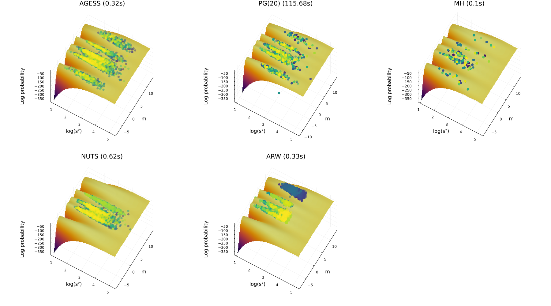

We can see that AGESS is able to traverse the multimodal distribution and efficiently sample from the posterior distribution. Notably, the particle gibbs sampler (PG) was able to also traverse the multimodal distribution; however, we can see that the sampler is significantly more computationally expensive, and is less efficient than AGESS (even though the same number of MCMC iterations were run). Similarly, the proposal kernel in the Metropolis Hastings sampler was diffuse enough to allow the sampler to traverse the different modes while being computationally fast to compute. However, we can see that the effective number of samples is significantly smaller than that of AGESS. Alternatively, the two adaptive sampling schemes that contain globally learned parameters (NUTS and ARW) were unable to effectively traverse the target distribution.

One cautionary takeaway is that users should not solely rely on ESS as a measure of a sampler's performance–-particularly when the target distributions are complex. From the graph below, if one were only to look at measures of ESS per second and disregard AGESS, one may conclude that NUTS would be the best sampler in this situation, despite the fact (unbeknownst to the user) that NUTS has trouble exploring the posterior distributions, and may not come close to reaching the stationary distribution in the finitely many iterations of the Markov chain.

function ess_per_sec_by_param(chain)
    s = MCMCChains.ess(chain)
    idx = Dict(p => i for (i, p) in enumerate(s.nt.parameters))
    return (s² = s.nt.ess[idx[Symbol("s²")]] / MCMCChains.wall_duration(chain),
            m = s.nt.ess[idx[:m]] / MCMCChains.wall_duration(chain))
end

chains = ["AGESS" => chain, "PG" => c1, "MH" => c2, "NUTS" => c3, "ARW" => c4]

samplers = first.(chains)
ess_matrix = reduce(vcat, [[ess_per_sec_by_param(ch).s² ess_per_sec_by_param(ch).m] for (_, ch) in chains])

n = length(samplers)
xs = 1:n
w = 0.35

p = bar(xs .- w/2, ess_matrix[:, 1]; bar_width=w, label="s²",
        xticks=(xs, samplers), yscale = :log10, ylabel="ESS / second",
        title="ESS per Second by Parameter and Sampler", yticks = [1, 10, 100, 1_000, 10_000], ylims = [1, 10_000])
bar!(p, xs .+ w/2, ess_matrix[:, 2]; bar_width=w, label="m", yscale = :log10)
p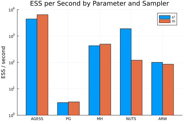

Key Takeaway: AGESS is locally adaptive and gradient free, which allows it to handle targets that have rapidly changing gradients (should they exist). However, the sampler is still also able to make global moves, allowing it to effectively traverse multimodal distributions.

# Free the sampled chains and cached plot surfaces before the next tutorial's page is built.
chain = c1 = c2 = c3 = c4 = chains = nothing
p_base = p = p1 = p2 = p3 = p4 = nothing
GC.gc()

This page was generated using Literate.jl.